When Does Longer Reasoning Help?

GitHub | Dataset

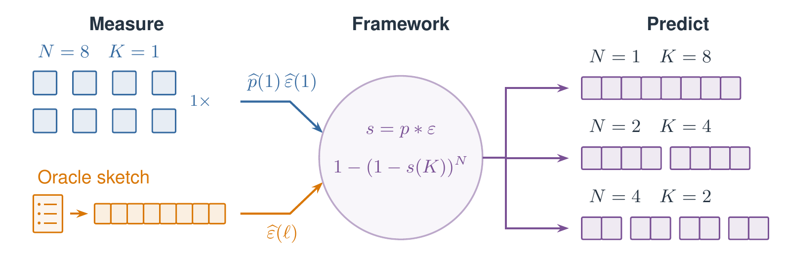
Short independent attempts and sketch-conditioned runs estimate discovery and execution, which together predict success when the same compute budget is split across different numbers of attempts.

Suppose an AI Agent has been working on a hard math problem for a while without solving it. Should we let it keep thinking, or start a fresh attempt? A longer attempt can finish an argument that is already on the right track. A fresh attempt may find an alternate approach that the first one missed.

We studied whether this tradeoff can be forecasted before running the longer attempts. Our framework, Discovery–Execution (DE), separates two parts of solving a problem: finding a viable proof strategy and turning that strategy into a complete proof.

Finding the Idea and Finishing the Proof

Anyone who has worked on olympiad combinatorics problems knows the distinction that it might take an hour looking for the right invariant, but, once it’s found the proof takes five minutes. On another problem, you know that you have to do Vieta jumping, but making the argument rigorous takes most of the work. These two show different bottlenecks of strategy discovery and conditional execution. Two models can have the same success rate under a short budget while facing different bottlenecks. Hence, the success rate alone does not tell us how much longer reasoning will help.

This intuition can be made rigorous with the following setup. Let $p(k)$ be the probability of first discovering a viable strategy in block $k$, and let $\varepsilon(\ell)$ be the probability of completing it within $\ell$ blocks, counting the discovery block. Then

We sum over when the idea arrives and how much time remains to execute it. This assumes execution depends on the available time, rather than when discovery happened.

Estimating the Parameters

For each problem and model, we run 24 independent one-block attempts. If $u$ succeed, our estimate of fresh success is $\widehat q=u/24$. Separately, we run three trajectories initialized with a verified strategy sketch of at most 25 words. If $v(\ell)$ have completed the proof by block $\ell$, then

In particular, $\varepsilon(1)$ is the probability of finishing the proof in one block given that the strategy is already available. It measures how reliably the model can execute the idea within that budget. We assume that executing a supplied strategy approximates executing one the model discovers itself.

We model discovery as geometric, with probability $\alpha$ of finding a viable strategy in each block, conditional on not having found one yet:

To solve within the first block, the model must both discover a strategy and execute it. Setting $K=1$ in the convolution gives

So fresh success alone underestimates discovery whenever execution can fail. Dividing out first-block execution gives the basic estimate, provided $\widehat\varepsilon(1)>0$:

For example, if $\widehat q=1/3$ and $\widehat\varepsilon(1)=2/3$, then $\widehat\alpha=1/2$: the model finds a viable strategy about half the time, but completes only two-thirds of those within the first block. These estimates give the longer-budget prediction

When fresh success exceeds measured first-block execution, the constrained fit also adjusts the execution estimate. With only three sketch-conditioned runs per problem, these estimates can be noisy. Our regularized version, R-DE, uses shared Beta and Dirichlet priors for discovery and execution timing, fitted across problems separately for each model. All fitting uses only these measurement runs; the longer unaided runs and alternate allocations are held out.

What We Found

We introduce AOBench: 35 hard, non-geometry problems from 2026 olympiads, each with a human-checked reference proof and strategy sketch. Together with 22 non-geometry problems from IMO-ProofBench Advanced, this gives 57 problems. We evaluate four models with three seeds per problem, or 171 trajectories per condition. Each compute block allows 200,000 output tokens, up to eight blocks.

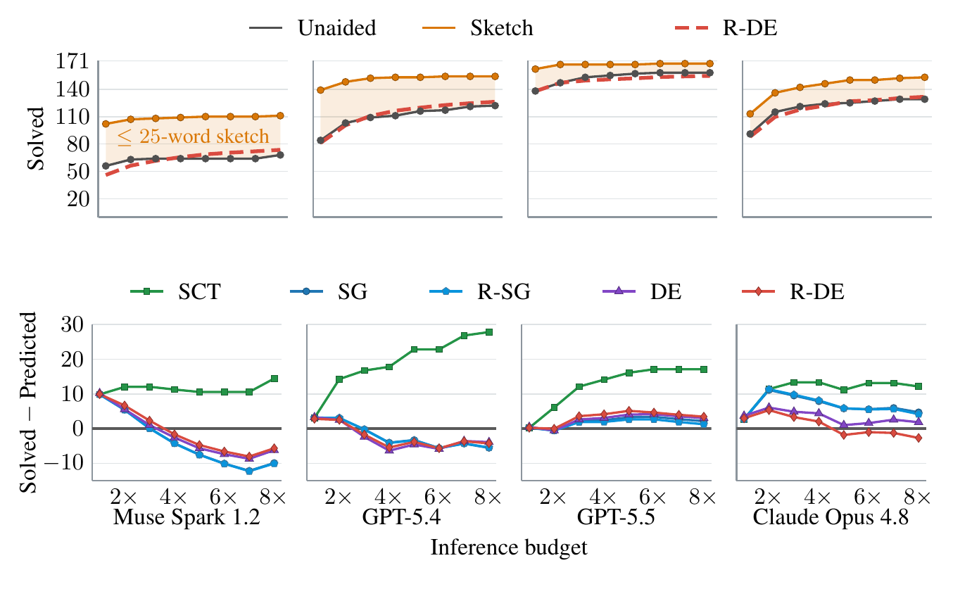
Top: success with a strategy sketch (orange), unaided success (gray), and R-DE predictions (dashed red). Bottom: observed minus predicted solved counts; closer to zero is better. SG is the simple geometric baseline, R-SG its regularized version, and SCT transfers the sketch curve’s gains directly to unaided success.

GPT-5.5 solves 162 of 171 sketch-conditioned trajectories within one block, increasing to only 168 after eight. Once it has the idea, execution is nearly saturated. Our DE Framework predicts that in such cases a simple geometric model, which treats each block as another chance of success, predicts its scaling curve well.

Claude Opus 4.8 behaves differently. Even with the strategy supplied, its successes rise from 113 to 153. Execution takes time. Accounting for this reduces prediction RMSE from 7.16 to 2.87 solved trials for one long attempt, and from 9.16 to 2.96 for two parallel attempts. These longer unaided runs were held out when fitting the predictors.

Predicting Alternate Allocations

The same measurements also predict success when we split the compute budget between two independent attempts ($N=2$). These alternate-allocation runs are held out as well; we do not refit the framework to their outcomes.

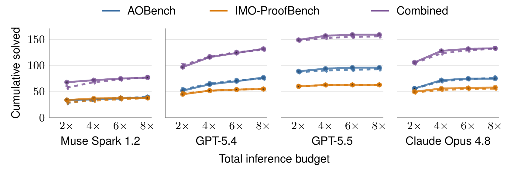
Solid curves show observed success and dashed curves show R-DE predictions for $N=2$. Colors separate AOBench, IMO-ProofBench, and their combined results. The horizontal axis counts the total budget across both attempts.

Across the four models, R-DE’s prediction RMSE for this allocation is 3.76 solved trials, compared with 5.84 for the simple geometric baseline.

The framework predicts aggregate behavior; it does not reveal a model’s internal reasoning. Still, the distinction is useful. Longer reasoning can help a model find an idea, finish an idea, or both. Measuring these separately gives us a better basis for deciding how to spend the next block of compute.